Testing Trading Strategies on Neighbouring Timeframes the Right Way
Robust timeframe testing is not about opening the same strategy on a higher or lower chart and hoping the equity curve still looks good. If the strategy uses indicator periods, bar-based filters, validity windows, or exit-after-bars logic, those values must be recalculated to preserve the same time exposure. Otherwise, you are not validating the same idea on a nearby timeframe — you are testing a materially different strategy.
This is the key principle behind proper neighbouring-timeframe validation. A 100-bar lookback on M15 does not represent the same market memory as a 100-bar lookback on H1. The first one covers 1,500 minutes. The second covers 6,000 minutes. That is a fourfold change in the amount of market history driving the signal. So when traders move a strategy from one timeframe to another without recalculating bar-based periods, they often believe they are testing robustness when they are actually testing parameter drift.
Why Period Recalculation Matters
The correct logic is simple:
new_period = old_period × (old_timeframe_minutes / new_timeframe_minutes)
That keeps the same underlying time horizon. For example:
- A 396-bar structure filter on M15 covers 396 × 15 = 5,940 minutes, or 99 hours.
- The equivalent on H1 is 99 bars, because 99 × 60 = 5,940 minutes.
This is exactly what you want: the strategy still “looks back” across the same amount of market time even though the chart resolution changed.
What Was Actually Tested Here
The supplied files contain four complete neighbouring-timeframe case studies with backtest exports:
- DAX strategy around an M15 base, tested on M10 and M30
- Dow Jones breakout strategy around an M5 base, tested on M1 and M15
- USDJPY momentum strategy around an M15 base, tested on M10 and M30
- XAUUSD volatility-compression strategy around an M30 base, tested on M15 and H1
These are exactly the kinds of tests that matter in real robustness work: one step lower and one step higher than the native timeframe, with parameter logic adapted to preserve time equivalence.
Strategy-by-Strategy Analysis of the Period Recalculation
| Strategy | Base TF | Lower TF | Higher TF | Recalculated bar-based periods | Unchanged price-space parameters | Interpretation |
|---|---|---|---|---|---|---|
| DAX MACD-RSI breakout filter | M15 | M10 | M30 | RSI 60 vs 20; MACD signal 24 vs 8; structure period 832 vs 278 | 5.4% profit target and ATR-based stop coefficient left unchanged | Most bar-based lookbacks compress almost exactly 3:1 between M10 and M30 |
| Dow Jones Vortex/LinReg breakout | M5 | M1 | M15 | Vortex 150 vs 10; LinReg 205 vs 14; Highest 1700 vs 113; BarsValid 30 vs 2 | TP/SL percentages unchanged; ShortExitAfter stayed fixed at 27 bars | Lookbacks are scaled close to 15:1, but the unchanged bar-exit materially changes real holding time |
| USDJPY RSI-MACD momentum | M15 | M10 | M30 | RSI 45 vs 15; structure period 390 vs 130; ExitAfterBars 86 vs 28 | 3% target and 20 pip stop left unchanged | Most core timing parameters scale about 3:1 between M10 and M30 |
| XAUUSD volatility compression breakout | M30 | M15 | H1 | StdDev 60 vs 15; Bollinger period 100 vs 25; structure period 396 vs 99 | Profit target 3225, stop 2140 and trailing stop 550 left unchanged | This is the cleanest example of exact time normalization: all bar-based periods scale 4:1 |
1) DAX MACD-RSI breakout filter
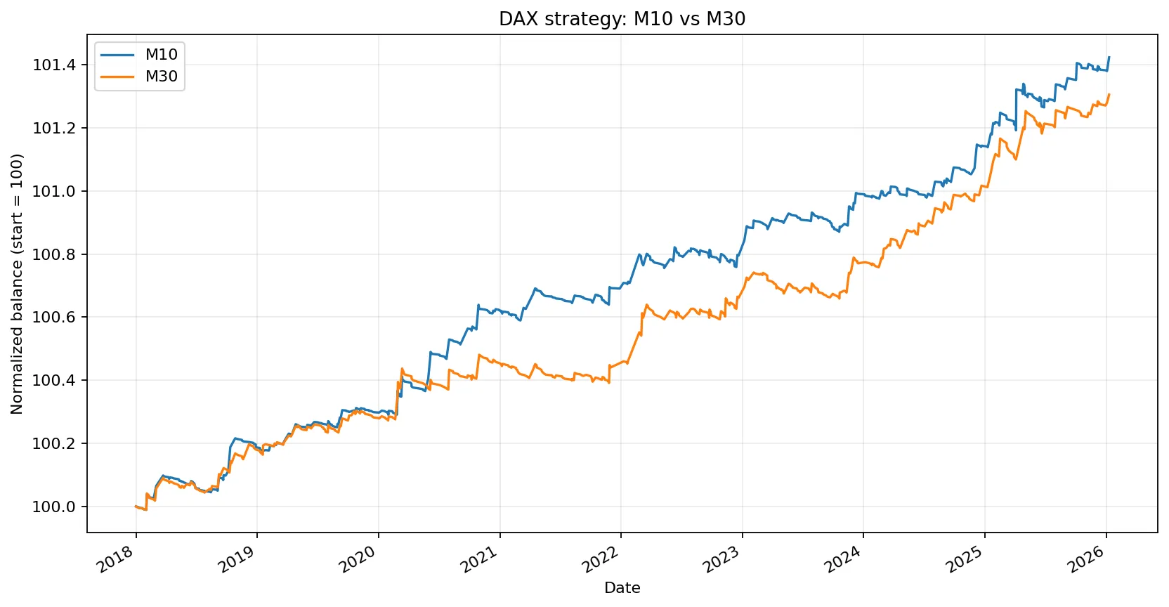
This strategy combines MACD timing, RSI filtering, and a very long structural lookback. The clearest normalization is visible in the long-period filter: 832 bars on M10 versus 278 bars on M30. In clock time, that is roughly 138.7 hours versus 139.0 hours — almost identical. RSI and MACD signal smoothing were also scaled in the expected direction, while the profit-target and ATR stop coefficient stayed unchanged because they work in price space rather than time space.
The interesting nuance is that one MACD leg remained fixed at 10 in both variants. That means the strategy is not a mathematically perfect bar-for-bar translation, but it is still close enough to preserve the character of the original logic. The backtest results confirm that the behaviour remained very stable.
2) Dow Jones Vortex/LinReg breakout
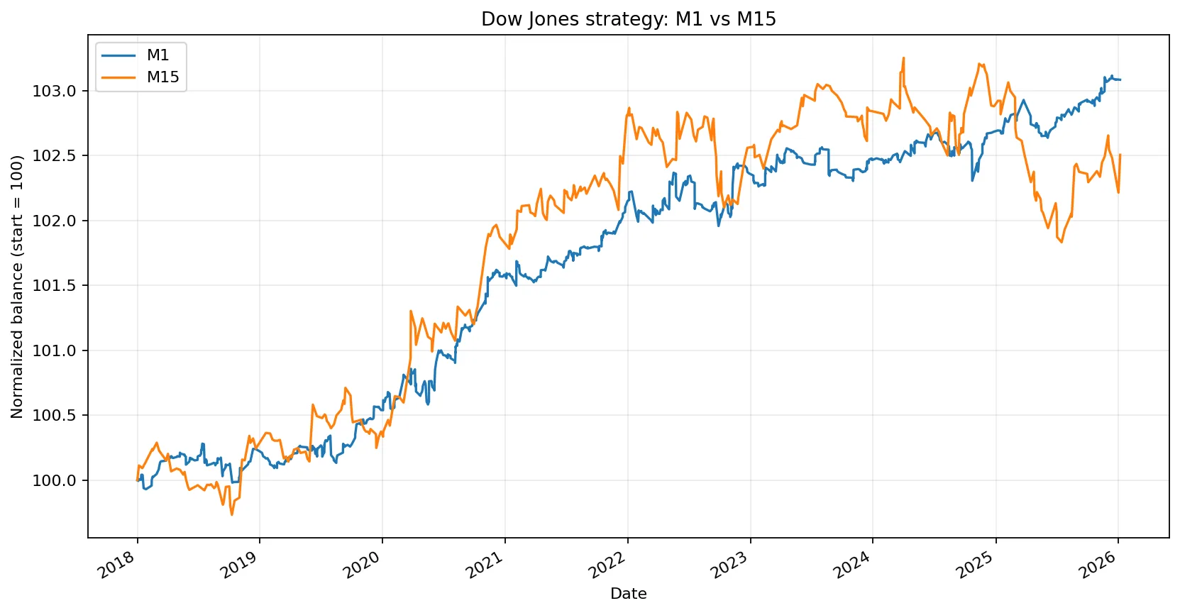
This is the best illustration of both proper scaling and the danger of partial scaling. Most of the bar-based parameters were translated very cleanly: LongVortexPeriod 150 vs 10, LongHighestPeriod 1700 vs 113, and ShortBarsValid 180 vs 12. These ratios are very close to the 15:1 relationship between M1 and M15. In other words, the strategy preserves the same time horizon for most signal components.
But one parameter stands out: ShortExitAfter stayed fixed at 27 bars in both variants. On M1 that means roughly 27 minutes. On M15 it means 405 minutes, or 6 hours and 45 minutes. That is a major behavioural change. It is a likely reason why the higher-timeframe version diverged more strongly in drawdown, Sharpe ratio, and trade distribution.
3) USDJPY RSI-MACD momentum
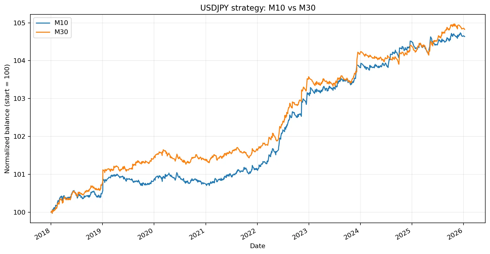
This is the cleanest M15-based translation in the set. The long structural filter moved from 390 bars on M10 to 130 bars on M30, which preserves exactly 65 hours of market memory. RSI moved from 45 to 15, and the exit-after-bars value moved from 86 to 28, again staying close to a 3:1 relationship. Fixed price-space parameters such as the 3% target and the 20-pip stop were kept unchanged, which is consistent with proper normalization practice.
The resulting performance is extremely similar across both neighbouring timeframes, which is exactly what you want to see when the underlying trading logic is truly robust.
4) XAUUSD volatility-compression breakout
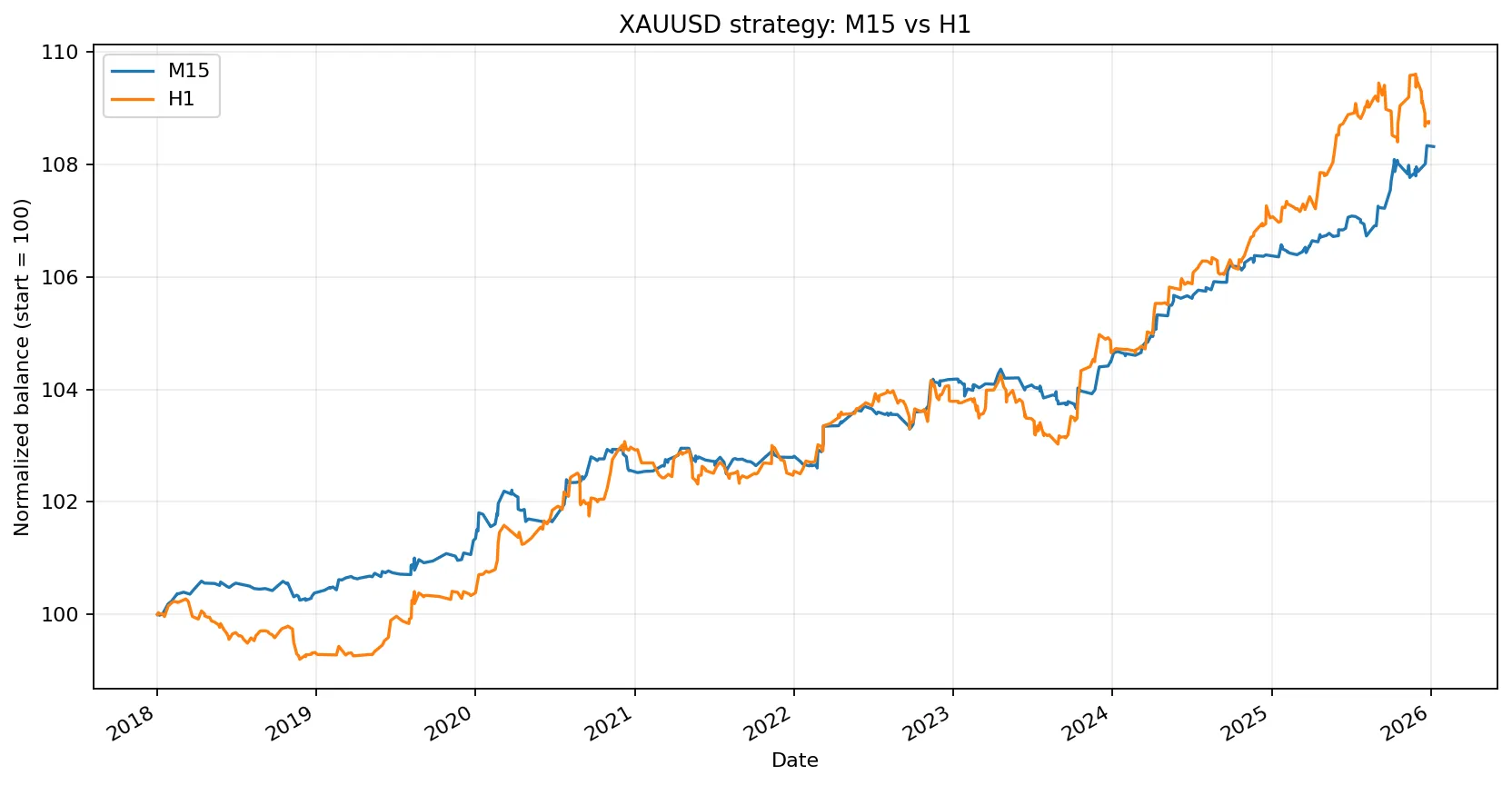
This is the cleanest textbook example of period normalization in the whole sample. StdDevFallingPeriod 60 vs 15, Bollinger period 100 vs 25, and structure period 396 vs 99 all follow the exact 4:1 ratio between M15 and H1 around the M30 base. In time terms, the strategy is reading the market through the same horizon on both neighbouring frames.
The fixed price-space controls — profit target, stop loss, and trailing stop — stayed identical, which is the correct approach for this type of volatility-compression system. The backtests remained profitable on both sides, but the higher timeframe produced wider equity swings and a lower profit factor, showing that correct normalization does not guarantee identical distribution.
Why Backtest Deviations Still Happen Even When Periods Are Recalculated
Even perfectly normalized strategies will not produce perfectly identical backtests. That is normal. A nearby timeframe changes the way price action is sampled, and that creates several unavoidable sources of drift:
Bar aggregation effect
Higher timeframes compress intrabar path. Stops, breakouts, pullbacks, and pending-stop entries may be triggered in a different order inside one larger candle than they would be on multiple smaller candles.
Integer rounding
Period translation is rarely perfectly divisible. A target value of 13.3 bars has to become 13 or 14. Across many signals, those small approximations accumulate.
Indicator kernel differences
EMA, MACD, Bollinger Bands, and standard deviation are not perfectly linear under resampling. A scaled period preserves approximate time exposure, but not an identical indicator shape.
Execution granularity
Breakout systems are especially sensitive. A pending stop placed above structure on M10 is not the same event as a pending stop placed above a candle defined on M30 or H1.
So the right question is not, “Did I get the exact same equity curve?” The right question is, “Did the strategy remain recognizably profitable, stable, and behaviourally consistent after proper time normalization?”
Equity Curve Comparison
Backtest Results Overview
| Strategy | Base TF | Test TF | Variant | Net Profit ($) | Profit Factor | Equity DD Max (%) | Trades | Win Rate (%) | Expected Payoff | Recovery Factor | Sharpe |
|---|---|---|---|---|---|---|---|---|---|---|---|
| DAX MACD-RSI breakout filter | M15 | M10 | Lower neighbouring TF | 142.32 | 1.98 | 0.09 | 741 | 15.25 | 0.192 | 15.01 | 4.89 |
| DAX MACD-RSI breakout filter | M15 | M30 | Higher neighbouring TF | 130.49 | 1.79 | 0.10 | 542 | 23.43 | 0.241 | 12.66 | 4.01 |
| Dow Jones Vortex/LinReg breakout | M5 | M1 | Lower neighbouring TF | 308.47 | 1.38 | 0.48 | 890 | 47.64 | 0.347 | 6.31 | 5.18 |
| Dow Jones Vortex/LinReg breakout | M5 | M15 | Higher neighbouring TF | 250.62 | 1.21 | 1.46 | 363 | 42.15 | 0.690 | 1.67 | 1.42 |
| USDJPY RSI-MACD momentum | M15 | M10 | Lower neighbouring TF | 463.75 | 1.38 | 0.35 | 1305 | 36.63 | 0.355 | 12.72 | 3.22 |
| USDJPY RSI-MACD momentum | M15 | M30 | Higher neighbouring TF | 482.67 | 1.43 | 0.41 | 1234 | 37.93 | 0.391 | 11.63 | 3.48 |
| XAUUSD volatility compression breakout | M30 | M15 | Lower neighbouring TF | 831.36 | 1.86 | 0.78 | 407 | 52.09 | 2.043 | 10.39 | 6.14 |
| XAUUSD volatility compression breakout | M30 | H1 | Higher neighbouring TF | 875.68 | 1.51 | 1.34 | 490 | 52.86 | 1.787 | 6.25 | 3.43 |
Deviation Summary Between Lower and Higher Neighbouring Timeframes
| Strategy | Base TF | Lower TF | Higher TF | Net Profit Δ | Profit Factor Δ | Equity DD Δ | Trades Δ | Win Rate Δ |
|---|---|---|---|---|---|---|---|---|
| DAX MACD-RSI breakout filter | M15 | M10 | M30 | -8.31% | -9.49% | +11.11% | -26.86% | +8.18 pp |
| Dow Jones Vortex/LinReg breakout | M5 | M1 | M15 | -18.75% | -12.50% | +204.17% | -59.21% | -5.49 pp |
| USDJPY RSI-MACD momentum | M15 | M10 | M30 | +4.08% | +3.48% | +17.14% | -5.44% | +1.30 pp |
| XAUUSD volatility compression breakout | M30 | M15 | H1 | +5.33% | -18.92% | +71.79% | +20.39% | +0.77 pp |
Interpreting the Results
- USDJPY was the cleanest robustness pass. The M10 and M30 variants delivered almost identical behaviour: net profit changed by only +4.08%, profit factor improved slightly from 1.38 to 1.43, drawdown moved only from 0.35% to 0.41%, and the trade count changed by just -5.44%.
- DAX also held up well. Net profit changed by -8.31% and profit factor by -9.49%, while equity drawdown stayed almost unchanged at 0.09% versus 0.10%.
- XAUUSD remained profitable on both sides of the base timeframe, but the distribution changed more visibly. H1 achieved higher net profit, yet profit factor dropped from 1.86 to 1.51 and maximum equity drawdown rose from 0.78% to 1.34%.
- Dow Jones stayed profitable, but this was the weakest neighbouring-timeframe translation. Net profit declined by -18.75%, profit factor by -12.50%, and maximum equity drawdown expanded by +204.17% from 0.48% to 1.46%.
Viewed together, these tests show something important: properly recalculated neighbouring-timeframe tests do not need to be identical to be valid. What matters is whether the core edge survives. In this sample, the DAX and USDJPY systems pass comfortably. XAUUSD passes with moderate distribution drift. Dow Jones is still profitable, but the drift is large enough to trigger a review of the time-normalization logic, especially around bar-based exits.
What Counts as an Acceptable Deviation?
There is no single universal threshold, because robustness depends on strategy style, market, and execution model. Still, in practical portfolio development, the following framework is a useful guide for neighbouring-timeframe validation after proper period recalculation:
| Metric | Excellent / Very Clean | Usually Acceptable | Warning Zone |
|---|---|---|---|
| Net Profit difference | within about ±10% | roughly ±10% to ±20% | above ±20% to ±25% unless compensated elsewhere |
| Profit Factor difference | within about ±5% to ±10% | roughly ±10% to ±20% | above ±20% |
| Maximum drawdown difference | up to about +20% to +30% | roughly +30% to +60% | above +60%, especially if profit factor also drops |
| Trade count difference | within about ±10% to ±25% | roughly ±25% to ±50% | above ±50% unless the strategy is intentionally intrabar-sensitive |
| Win rate difference | within about ±2 to ±4 percentage points | roughly ±5 to ±8 percentage points | above ±8 percentage points without offsetting improvement elsewhere |
Final Conclusion
The main lesson is straightforward: testing a strategy on neighbouring timeframes only makes sense when bar-based periods are recalculated into equivalent market time. Without that step, the test does not measure robustness. It measures how a different strategy behaves on a different chart.
When this normalization is done correctly, small and medium deviations are completely normal. In practical terms, a very good neighbouring-timeframe pass often stays within roughly 10% on net profit, 5%–10% on profit factor, and 20%–30% on drawdown. Broader but still usable robustness usually falls inside about 20% on net profit and 30%–60% on drawdown, provided the edge remains clearly positive. Once multiple metrics deteriorate together — especially when drawdown expands sharply and trade behaviour changes dramatically — the strategy should be treated as only partially transferable or not robust enough for timeframe migration.
In this sample, USDJPY and DAX show the strongest neighbouring-timeframe robustness, XAUUSD shows an acceptable but looser transfer, and Dow Jones highlights exactly why every time-based component must be normalized carefully, including exit horizons. That is the real takeaway: neighbouring-timeframe testing is not about finding a prettier equity curve. It is about proving that the edge survives when chart resolution changes but market-time logic remains consistent.